Using Geospatial Models For Estimating And Projecting Population For Small Areas

• Rich Doty, MA, GIS Coordinator & Research Demographer, BEBR

Population forecasts for small areas (e.g., traffic analysis zones, school zone, neighborhoods, zip codes) often play an important role in public and private sector decision making.  They are essential in planning for future needs related to transportation, education, housing, emergency services, utilities, water resources, climate change, health care, local government planning, and many other goods and services.

The University of Florida’s Bureau of Economic and Business Research (BEBR), through a contract with the Florida Legislature, annually produces Florida population numbers, both estimates of current population and projections of future population. However, the estimates are available at the state, county and city levels, and the projections are available at the state and county levels. Because population estimates and projections are often needed for smaller areas, BEBR also produces them on a contract basis. This article is an overview of BEBR’s approach to developing small-area population projections.

To project population for small areas, physical constraints should be considered. For example, if a small area (e.g., census tract) has experienced a historically high rate of growth but has no more land available for residential development, projecting growth for that area based on the historical trend would overstate the future population for that area. Although potential future redevelopment and/or increased occupancy rates could result in some growth, the projection should be limited by the future development potential of that area. Moreover, physical features such as roads can influence where future growth occurs. For these reasons, we use geospatial models (models built using Geographic Information System, or GIS, software and data) that are capable of accounting for these important considerations to develop our small-area projections.^[1]

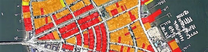
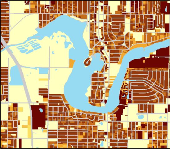
Our geospatial models are built using property parcel data from county property appraisers. These data include the property parcel boundaries and attributes that indicate the property use, the number of residential units, the year the residences were built, and the lot size. To this we add data from other sources that enable us to project maximum development potential (or “build-out”) at the parcel level, including

• Population, average household size and average occupancy from the 1990, 2000 and 2010 decennial censuses
• Future land use classification and unit densities from local government future land use maps
• Surface water and wetlands
• Conservation lands and other areas for which development is restricted
• Planned development boundaries and approved residential units
• Redevelopment area boundaries and net change in residential units (where available)
• Any political, natural or other boundaries needed for summarizing the results (cities, utility boundaries, traffic analysis zones, watersheds, school zones, etc.)^[1]

Using this “Build-out Submodel” (depicted in Figure 1), we can also estimate current population. We apply average household size and occupancy metrics from the 2010 Census (with occasional adjustments using trends in the American Community Survey) to the parcel-level residential unit estimates provided by the county property appraisers. We then add population in group quarters (e.g., nursing homes, college dormitories, prisons) and summarize these population estimates by city and county. Finally, we make any minor adjustments to control the current population to our published population estimates^[3] for Florida’s cities and counties derived using different models.

To project future growth, we start by calculating historic growth trends. While the methods and data can vary, these are typically based on tract-level data from the 1990, 2000 and 2010 censuses and our current estimates. These data are used to produce 12 tract-level projections using six different demographic extrapolation methods over multiple base periods. The highest four and lowest four calculations are discarded to moderate the effects of extreme projections.^[3] The remaining four projections are then averaged. The six demographic extrapolation methods for projecting population we currently use include

1. Linear – the change in the number of persons for each census tract will be the same in future years as the average annual change during the base period.^[4]
2. Exponential – that population will continue to change at the same percentage rate in future years as the average annual rate during the base period.^[4]
3. Constant Population – future population will remain constant at its current value.^[5]
4. Constant-Share – each census tract’s percentage of the county’s total population will be the same as the average percentage during the base period.^[6]
5. Share-of-Growth – each census tract’s percentage of the county’s total growth will be the same as it was during the base period.^[4]
6. Shift-Share – each census tract’s percentage of the county’s total annual growth will change by the same annual amount as the average annual change during the base period.^[4]

Figure 1. Build-out Submodel depicting housing units per acre in Tampa, Florida.

The Linear, Exponential, and Constant Population techniques employ a bottom-up approach, extrapolating the historic growth trends or population of each census tract with no consideration for the county’s overall growth. The Constant-Share, Share-of-Growth, and Shift-Share techniques employ a ratio allocation, or top-down approach, allocating a portion of the total projected county population or growth to each census tract based on that census tract’s percentage of county population or growth over the historical period.

Each of the six methods is a good predictor of growth in different situations and growth patterns, so using a combination of all six is the best way to avoid the largest possible errors resulting from the least appropriate techniques for each census tract when developing small-area forecasts over large regions.^[7] This approach is similar to the one BEBR uses for the county population projections, but because annual estimates are not available at the tract level, the base periods and the number of projections are somewhat different.

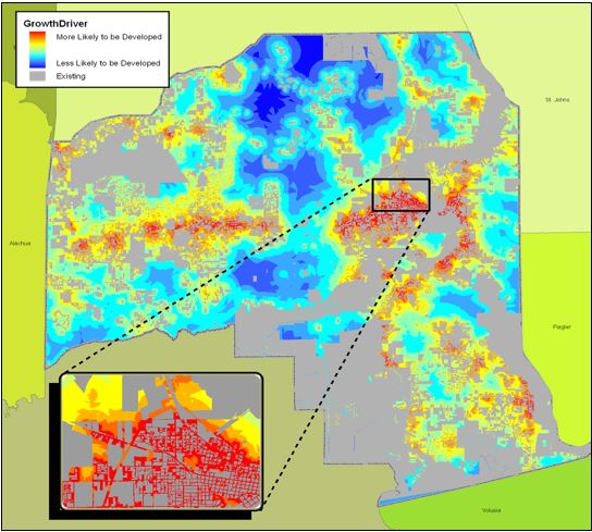
In addition to historic growth trends, spatial features can influence future growth. For that reason, we determine the historical relationship between residential development over the past 20 years and its proximity to the following features:

1. Roads and interchanges prioritized by level of use (with each road type modeled separately)
2. Existing residential development
3. Existing commercial development (based on parcels with commercial land use codes deemed attractors to residential growth)
4. Coastal and inland waters
5. Large planned developments

The results of multiple logistic regressions are combined into a single “Growth Drivers Submodel” extending beyond the area to be projected to eliminate edge effects. The values are reclassified into 10 classes, with 10 indicating the highest likelihood for development.^[1] An example of this is shown in Figure 2.

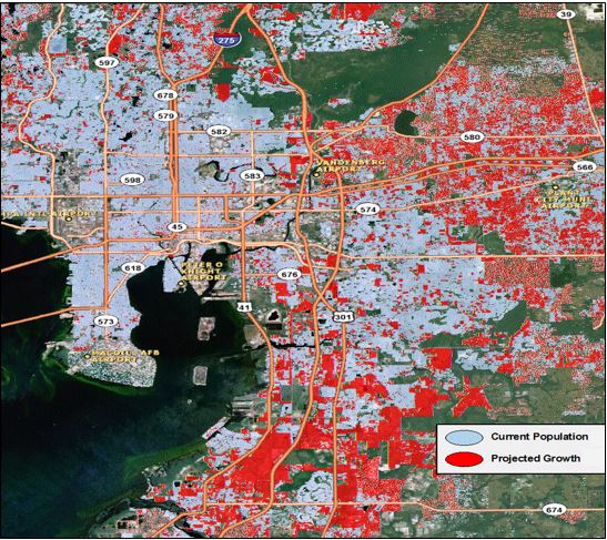
Projections are typically made in 5-year increments with approximately a 30-year horizon (2020, 2025, 2030, 2035, 2040, and 2045), although annual increments and longer horizons are possible. The projection derived from the growth trends for each tract is compared against the maximum development potential from the Build-out Submodel. This cap is based on the land available for residential development, the recent historical densities for which each land use in each jurisdiction have developed, any planned redevelopment, and any projected changes in occupancy. If the growth exceeds the capacity, the tract’s growth is limited to the capacity. Once this is done for all tracts in a county, the total of this preliminary county growth is compared against the published BEBR forecast for the county for that time period. While the projected growth is typically close to the published county projection, the growth can be adjusted to match the county number exactly. For downward adjustments, the growth is typically reduced for all tracts in proportion to their growth over the period. For upward adjustments, we use the Growth Drivers Submodel to identify groups of parcels with the highest relative growth probability for development.^[1] These upward adjustments are more common as we move further away from the current year, as more areas that are currently growing reach their maximum capacity.

Figure 2. Growth Drivers Submodel for Putman County, Florida

Like our population estimates and forecasts for the Florida Legislature and the census counts, these small-area population projections are of permanent residents only. We do have the ability in some areas to estimate and project seasonal, tourist, and commuter populations, but those are limited by data availability. Because the census tract-level growth is allocated to individual parcels, the process of summarizing the parcel-level results by any boundaries (e.g., cities, traffic analysis zones, school districts, neighborhoods, zip codes) is easier and more accurate than translating census tracts to different boundaries based on the proportion of the tract area falling within them. Project deliverables typically include GIS data (shown in Figure 3) with the parcel-level detail, and spreadsheet summaries of the results.

Figure 3. Current and projected population in Hillsborough County, Florida

Planning, permitting and resource considerations have elevated the importance of small-area population projections, particularly in areas experiencing rapid growth since the Great Recession. This methodology enables the development and regular updates of estimates and projections at any geographic level using the best available data and industry standard techniques and tools. Controlling the small area projections to our published county forecasts provide consistency with other projections made by state and local governments, while at the same time providing the spatial precision needed for those requiring small-area population estimates and projections.

Contact Rich Doty with questions about BEBR’s small-area population estimates and projections.

REFERENCES:

[1] Doty, Richard L. (2016), “The Geospatial Small-Area Population Forecasting (GSAPF) Model Methodology Used by the Southwest Florida Water Management District”. GIS Associates, Inc.  Gainesville, Florida.

[2]Bureau of Economic and Business Research (2016), “Florida Estimates of Population 2016.”  Bureau of Economic and Business Research, University of Florida. Gainesville, Florida.

[3] Smith, Stanley K., and Stefan Rayer (2004).  “Methodology for Constructing Projections of Total Population for Florida and Its Counties: 2003-2030.”  Bureau of Economic and Business Research, University of Florida. Gainesville, Florida.

[4] Rayer, Stefan, and Ying Wang (2017). “Projections of Florida Population by County, 2020-2045, with Estimates for 2016.”  Florida Population Studies, Bulletin 177, April 2017. Bureau of Economic and Business Research, University of Florida. Gainesville, Florida.

[5] Smith, Stanley K., and Stefan Rayer (2014). “Projections of Florida Population by County, 2015-2040, with Estimates for 2013.”  Florida Population Studies, Bulletin 168, April 2014. Bureau of Economic and Business Research, University of Florida. Gainesville, Florida.

[6] Rayer, Stefan (2015). Personal communication September 9, 2015. Bureau of Economic and Business Research, University of Florida. Gainesville, Florida.

[7] Sipe, Neil G., and Robert W. Hopkins (1984), “Microcomputers and Economic Analysis: Spreadsheet Templates for Local Government”, BEBR Monographs, Bureau of Economic and Business Research, University of Florida, Gainesville, Florida.